AI in baby steps, experiment 2: making your own Multilayer Perceptron (MLP), a real Deep Learning machine
- Ruwan Rajapakse
- Jan 24, 2025
- 7 min read

Spoiler: Excel file with VBA code and working 3-layered MLP included below!
Imagine for a moment that you are a manufacturer of riverboat engines. You produce several different models, known for their high quality and durability. With regular servicing, these engines can last for decades.
However, on occasion, an engine due for servicing may sputter and stop while running. You've observed that this typically occurs within a few minutes of startup, with subtle warning signs appearing shortly beforehand. For instance, the engine’s surface temperature might rise unusually high, or there could be excessive vibrations.
This brings up a question: is it possible to predict such failures in advance? Could a captain be alerted before heading out, preventing a breakdown in the middle of the river? Perhaps a simple software solution could be developed to run on an inexpensive single-board computer. This software could take inputs from temperature and vibration sensors on the engine and trigger a dashboard light if failure seems imminent, warning the captain to service the engine before departing.
You know the system will require two inputs—temperature and vibration readings taken five seconds after startup—and it will provide a single binary output. The output would trigger a red warning light when the system detects a potential failure (i.e., when the output is 1). You suspect that the thresholds for these inputs and the logic for predicting failure might vary between engine models. Nevertheless, you want to create a versatile piece of software that can intelligently learn the failure patterns for any given model.
In this experiment, we aim to build such a system. Let’s assume we’ve studied numerous failure scenarios for one specific engine model. For this model, we want to pilot the early warning system. We have collected 500 records, each containing vibration and temperature readings five seconds after startup, along with labels indicating whether the engine failed within five minutes. Below are the first ten records as an example.
Vibration (m/s^2) | Temperature (°C) | Engine Failure (Y) |
5.88662748 | 46.37639226 | 0 |
1.21280678 | 67.3582853 | 1 |
1.139695183 | 44.10620459 | 0 |
8.939113326 | 44.9837688 | 1 |
5.789178077 | 64.87518095 | 1 |
2.892620671 | 33.95070155 | 0 |
5.207101716 | 82.71468458 | 1 |
7.43261077 | 45.97053318 | 1 |
1.457435893 | 67.11169411 | 1 |
7.135809753 | 58.24687615 | 1 |
In our last experiment, we learned that a single perceptron can classify data points as belonging to a specific category (e.g., a rose) or not, but only if the data points are linearly separable in a multidimensional space called hyperspace. For example, the perceptron can distinguish roses from other objects when the features (or dimensions) of roses form a distinct cluster that can be separated by a straight line or hyperplane.
Now, let’s apply this concept to our current problem. We’ll plot the two inputs—vibration and temperature (x₁ and x₂)—against each other, labeling the pairs that lead to engine failure in green and those that don’t in red. Our goal is to observe whether we can draw a straight line (or hyperplane, in this 2D case) to separate the failure data from the non-failure data.

We’ve applied a simple but effective trick to make it easier to identify data clusters while maintaining the same scale for both axes in hyperspace. We’ve scaled the values of x₁ and x₂ to range between 0 and 1. This ensures the clusters are more visually distinguishable, without being compressed along one axis. As we’ll see later, scaling inputs—especially to a range of 0 to 1—is not only helpful for visualization but also plays an important role when we develop the neural network to solve this problem.
As you can see, the useful data points in green do form a noticeable cluster. However, there isn’t a single straight line that can separate this cluster from the rest. It seems we’d need a more complex boundary—such as two intersecting lines—defined by multiple mathematical functions to determine whether a given engine condition would lead to failure. In other words, this problem cannot be solved with a single perceptron.
Fortunately, there is a solution. We can stack and pack perceptrons up in layers to discover and memorize such complex boundaries! Let’s figure out how to do this.
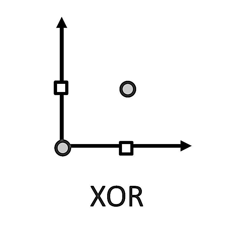
If you closely examine the clustering of the engine failure data, you’ll notice that the pattern resembles the logical XOR operation. Specifically, when x₁ is above a certain threshold and x₂ is below a certain threshold, the pair (x₁, x₂) predicts failure. Conversely, when x₁ is below its threshold and x₂ is above its threshold, the pair also predicts failure. However, if both x₁ and x₂ are either below or above their respective thresholds, the pair does not predict failure. This logic corresponds directly to the truth table of XOR.
As seen in the graph below, even if we simplify the situation by removing different threshold values and assume a threshold of 1 for both x₁ and x₂ —meaning that if either x₁ or x₂ is 1, but not both, the engine would fail—we still wouldn't be able to separate the XOR cluster of interest with a simple line.
However, a perceptron can detect simpler logical functions like AND or OR, which are linearly separable (see graphs below).

With this understanding, we can propose a conceptual architecture (see below) for a simple Multi-Layer Perceptron (MLP) to detect XOR. The network consists of three layers of neurons: an input layer with two nodes (placeholders for data), a hidden layer with two perceptrons, and an output layer with a single perceptron. The key idea is that the hidden layer allows the network to decompose the XOR problem into simpler, linearly separable components.

A brief explanation:
Input Layer: This layer contains no neurons and is just a conceptual representation of the two inputs x₁ and x₂.
Hidden Layer: This layer contains two neurons. Each neuron learns a distinct part of the XOR logic:
One neuron can learn the logical AND function, which activates when both inputs are 1. This data point cluster is linearly separable.
The other neuron can learn the logical NAND function, which activates when both inputs are 0 or when exactly one of the inputs is 1 (and not both). This data point cluster is also linearly separable.
Output Layer: This single neuron takes the outputs from the hidden layer and combines them. By learning to concatenate (or combine) the outputs of the two hidden neurons, it effectively constructs the XOR logic.
With this structure, the hidden layer decomposes the problem into two simpler functions, and the output layer recombines them to determine the XOR function. This demonstrates how adding a hidden layer makes it possible for neural networks to handle non-linear relationships in data.
Now that we’ve refreshed our understanding with some theory to aid in building our engine failure detector, let’s move on to developing it as an imperative codebase. As before, I’m using Excel and VBA to demonstrate visualizations and illustrate the steps involved in applying an MLP to solve the engine failure check light problem. This program is written for relatively inexperienced coders like me who want to gain a deep understanding of how neural networks work under the hood of popular machine learning libraries. The code works—albeit inefficiently—and it is thoroughly commented and aims to illustrate all the major steps in designing a feedforward neural network with backpropagation.
The MLP I've constructed is a 3-layer binary classifier, with flexibility to change the number of neurons in the input and hidden layers. Take a close look at the code image below. You can also download the Excel file and edit the attached VBA Macro yourself (see further down).

As you can see from the code comments, there is structure to the code that indicates a sequential set of initializations and matrix operations to be performed. These matrix operations look somewhat complex and tedious, simply because I'm implementing all of them from first principles, in keeping with our overall objective. If one used a machine learning library, the implementation at each step such as the forward pass would be way simpler, or even be entirely dispensed with (at the peril of losing sight of what exactly is going on).
To recap what's in the code, the five main steps are:
Initialization:
Define the architecture of the MLP (number of neurons in each layer).
Initialize the weights and biases for the layers.
Forward Propagation:
Calculate the outputs for each layer.
Apply activation functions to the hidden and output layers.
Loss Calculation:
Compute the difference between predicted output and actual output using a loss function.
Backward Propagation:
Compute gradients of the loss with respect to weights and biases using the chain rule.
Update weights and biases based on the gradients.
Training Loop:
Iterate through multiple epochs.
Perform forward propagation, loss calculation, backpropagation, and update the weights.
I hope this code provides valuable insights into the details of the implementation. I’d like to highlight a few new concepts introduced here that we didn’t encounter in our earlier experiment with simple perceptrons. These include:
Gradient descent.
Sigmoid and other activation functions, along with their relative merits.
The logic behind backpropagation.
Configuring an MLP for a specific problem (e.g., determining the number of hidden layer neurons, selecting an appropriate learning rate, etc.)
While there are many excellent blog posts and tutorials covering these topics, I’ll also share my own thoughts and perspectives in my next post.
Finally! Now we come to the crux of our entire discussion. I've attached below the Excel spreadsheet that simulates the engine failure app using an MLP. Please ensure you scan the file before use, as one can never fully guarantee the safety of files hosted on public servers.
When you tap the 'Discover Hyperplane' button, remember that you're running a computationally intensive algorithm in Excel. Please tap it only once and allow the code a few minutes to complete its process and update the graph on the right.
The graph on the right shows the contours of the hyperplane discovered by the MLP. As a stochastic process that learns from data, the MLP's output won't perfectly match the actual x₁ vs x₂ graph plotted manually (the graph on the left). However, it will come close. The MLP 'learns and remembers' these contours, enabling it to classify inputs. For instance, if we forward-pass a new pair of vibration and temperature values not present in the training data, the MLP will classify them as indicative of engine failure or not.
There’s still plenty of theory left to discuss, which I hope to tackle in my next post. After that, we’ll move on to building more complex ML constructs, this time leveraging established ML libraries. Meantime, happy experimenting!


Comments